Scaling Gaussian Splatting to Longer Contexts

• Ameya Javery
• Harsh Shah
• Sarayu Anantharaman

Motivation

3D reconstruction systems excel at either small-scale photorealism or large-scale sparse mapping, but rarely both. Over thousands of monocular frames, models run out of VRAM and suffer from scale drift.

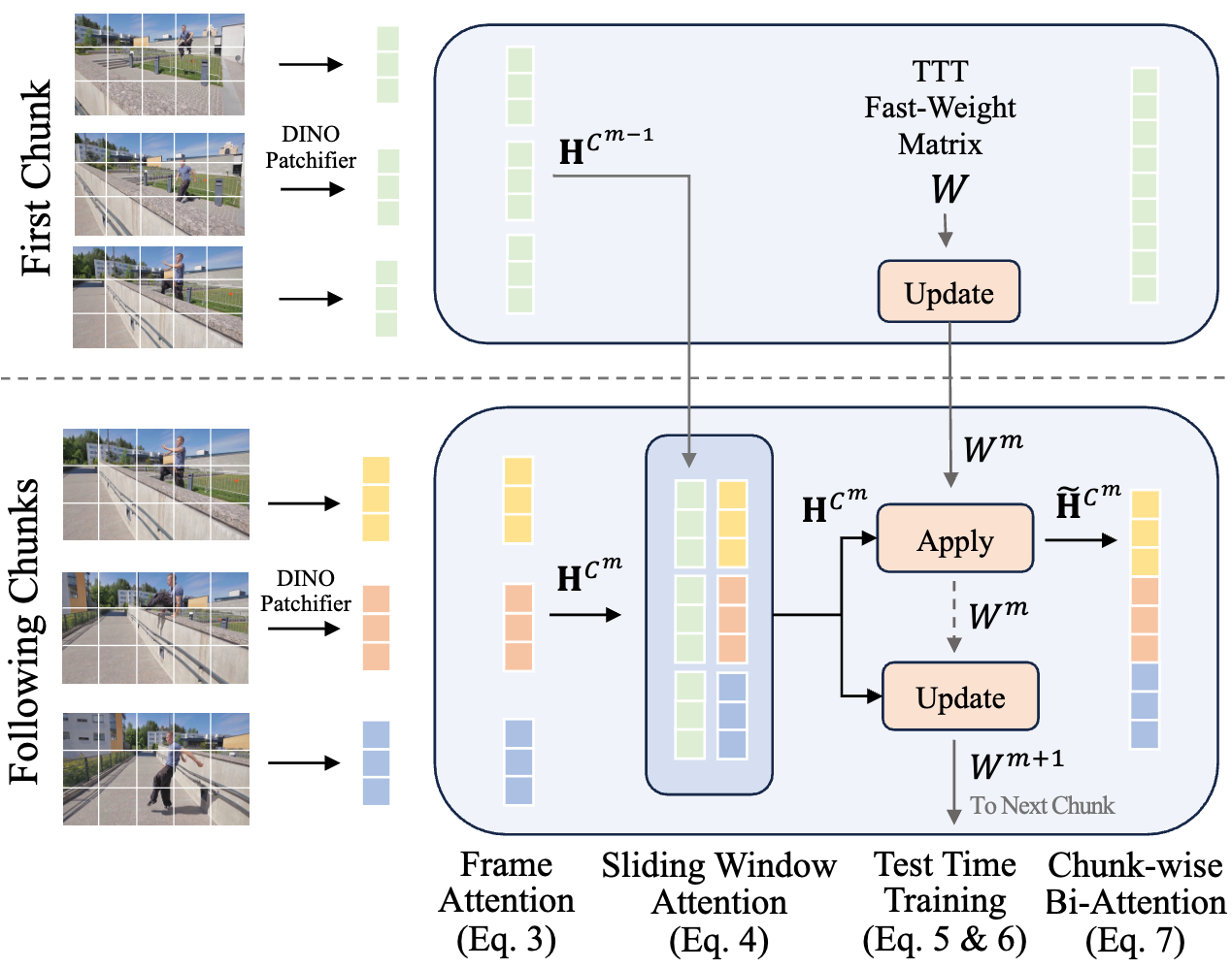
LoGeR (Long Context Geometric Reconstruction) mitigates a part of this. It uses a hybrid of two approaches: chunking frames and pairing local and lossless Sliding Window Attention with global, lossy Test-Time Training, yielding a globally consistent dense point cloud.

3D Gaussian Splatting adds the photorealism a point cloud generally lacks. It initializes Gaussians from the point cloud prior and optimizes their position, covariance, opacity, and color through differentiable rasterization against the input images. The bottleneck often is memory, since large scenes usually imply joint optimisation of millions of Gaussians.

Our central question is: can long-context, photorealistic 3D reconstruction run under a limited memory budget?

We hence target optimising this pipeline to construct a photorealistic digital twin of our college campus, running on a single RTX 4090 (24 GB VRAM).

A. Fixing the Geometry: LoGeR

LoGeR tackles three massive bottlenecks in long-video reconstruction:

1. Scale Drift: The gradual accumulation of minor errors in camera tracking over long distances. This leads to geometric inaccuracy, spatial distortion and a non-uniform global scale for objects.
2. The Context Wall: Full bidirectional attention over all frames costs quadratic $O(n^2)$ compute in the number of tokens.
3. The Data Wall: Long-video training datasets are scarce, and can cause models to fail on extended real-world inputs.

The solution implements a Hybrid Memory Mechanism that chunks video frames and sews them together using two distinct memory types.

Sliding Window Attention

A non-parametric, lossless mechanism that applies full scale bidirectional attention on a single chunk of frames. It deals in uncompressed data and acts as a local stitcher that aligns corners, edges, and textures perfectly.

Test Time Training

Across a huge number of chunks, gradually, the error in aligning the chunks accumulates and scale drift increases. As a result, the model would lose track of the overall scene.

Thus, TTT forms an overall map of the entire scene, keeping track of global scale and macro geometric details. TTT is a lossy, parametric memory map that tracks the entire scene. It has a set of internal fast weights, which are updated during inference as new chunks are processed.

The overlap between consecutive chunks provides shared information that helps TTT relate the new chunk to previously processed parts of the scene. Using this information, the fast weights are updated to maintain consistency in alignment and scale. This prevents small errors from accumulating as hundreds of local chunks are stitched together.

Deep dive

To better understand how each parameter affects LoGeR’s output, we ran the inference pipeline varying one parameter at a time and analysed the resulting reconstructions. LoGeR’s inference pipeline exposes six primary parameters:

1. Window size: The number of consecutive frames processed jointly as a single chunk.
2. Overlap size: The number of frames from the previous window that are retained in the next window.
3. TTT reset interval: The interval after which the TTT fast weights are reset to their initial state.
4. Stride: The temporal step between frames sampled from the input video.
5. Base learning rate: The step size for TTT fast-weight updates during inference.
6. Sim(3) scale mode: How relative scale between adjacent chunks is resolved when aligning them with a Sim(3) transform.

A larger window size reduced scale drift and jitter and increased mean and fractional confidence, while a smaller window size of 8 showing visible drift and an accommodable window size of 64 giving the best reconstruction.

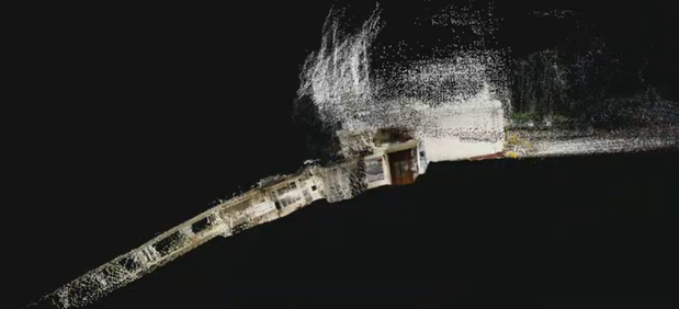
Increasing overlap raised confidence while scale drift stayed roughly constant. With zero overlap, the apparent scale drift was 0 because drift is not computed without overlap, and the full point cloud collapses into one place.

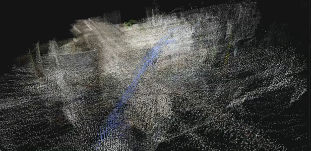
The confidence peaks at a TTT reset interval of 8 and drops at longer intervals, likely because the model overfits to previous windows and fails to adapt to later parts of the scene with different geometry and lighting.

Small strides caused jitter because closely spaced frames have small triangulation angles, which amplify pixel-level noise; larger strides reduced scale drift by reducing the number of chunks to stitch together, but lowered confidence as fewer input frames were used.

Best configuration

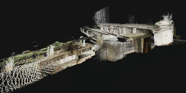
The best configuration used a window size of 64, an overlap of 12 to 16, and a TTT reset interval of 8.

B. To Recap 3D Gaussian Splatting

3D Gaussian Splatting represents a scene explicitly as a set of Gaussians. Each Gaussian has four learnable properties:

1. Position $\mu$: the center of the Gaussian in 3D space.
2. Covariance $\Sigma$: its shape and orientation, stored as a scale vector $S$ and a rotation quaternion $R$, with $\Sigma = R S S^\top R^\top$.
3. Opacity $o$: how much the Gaussian blocks light behind it.
4. Color $c$: stored as spherical harmonic coefficients, so color can change with viewing direction and model view-dependent effects like specular highlights.

Alpha blending

To render an image, each Gaussian is projected onto the image plane, where its 2D covariance is

\[\Sigma' = J W \Sigma W^\top J^\top\]

with $W$ as the world-to-camera transform and $J$ as the Jacobian of the projection. The screen is divided into 16×16 pixel tiles, and the Gaussians overlapping each tile are sorted by depth, front to back. The color of a pixel is then

\[C = \sum_{i=1}^{N} c_i \, \alpha_i \, T_i\]

where the effective opacity of Gaussian $i$ at pixel $x$ is

\[\alpha_i = o_i \exp\left(-\tfrac{1}{2}(x - \mu'_i)^\top \Sigma'^{-1}_i (x - \mu'_i)\right)\]

and the transmittance, the fraction of light that reaches Gaussian $i$ after passing through the ones in front of it, is

\[T_i = \prod_{j=1}^{i-1} (1 - \alpha_j)\]

Training

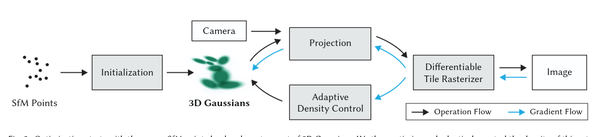
Each rendered view is compared against the ground-truth image from the same camera, and the gradients are backpropagated with Adam to update every Gaussian’s position, covariance, opacity, and color, while adaptive densification clones, splits, and prunes Gaussians as training progresses. The loss combines a per-pixel photometric L1 term with a D-SSIM term that compares local luminance, contrast, and structure:

\[\mathcal{L} = (1 - \lambda)\,\mathcal{L}_1 + \lambda\,\mathcal{L}_{\text{D-SSIM}}, \qquad \mathcal{L}_{\text{D-SSIM}} = 1 - \text{SSIM}, \qquad \lambda = 0.2\]

Tinysplat

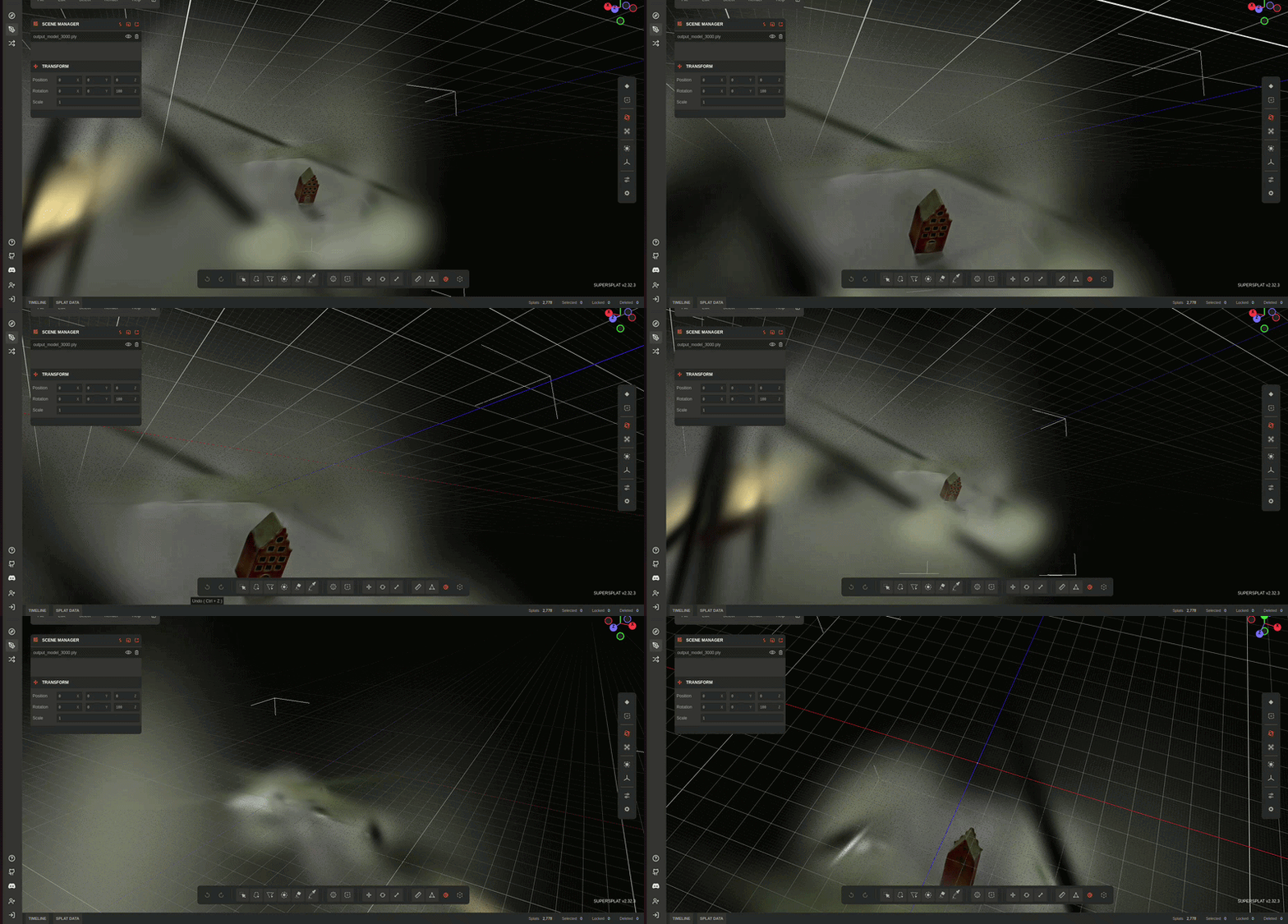
We built tinysplat, a from-scratch reimplementation of vanilla 3D Gaussian Splatting. Trained on a small object, it initially rendered only a dark outline. Increasing the Gaussian count from around 125 to 250 through more aggressive densification did not visibly improve the render. Hence we identified opacity resets as the bottleneck and removed them entirely, which produced a clear render of the object and became our final baseline.

Scaling Tinysplat

Our integration pipeline initializes 3D Gaussian primitives using LoGeR’s predicted point cloud. Surprisingly, despite the geometric accuracy of the point cloud prior, the early optimization steps resulted in severe visual degradation, producing unaligned and unrecognizable renders during rasterization.

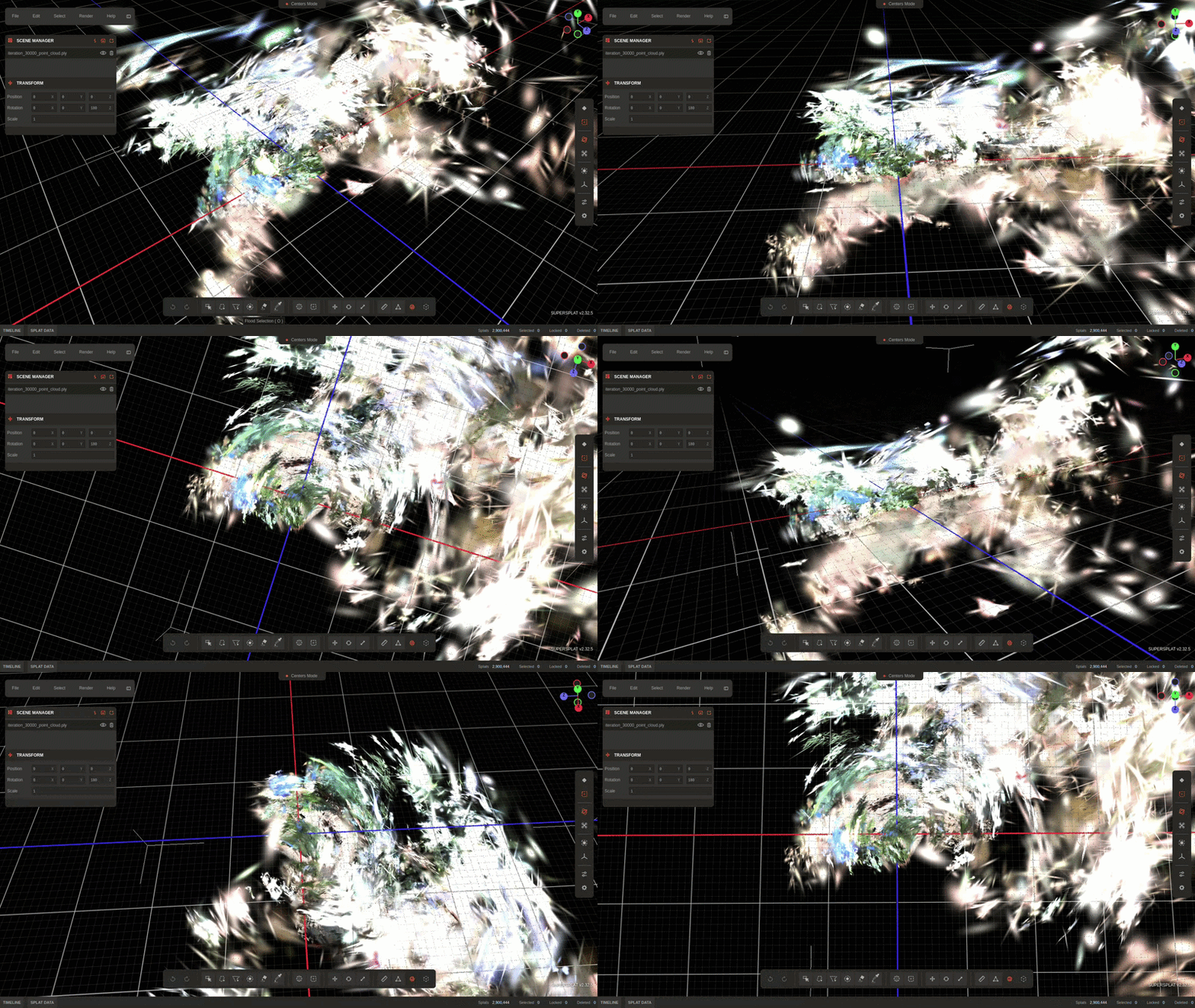
Our initial attempts hence exposed two bottlenecks. Jointly optimizing millions of Gaussians exceeds a single 4090’s 24 GB VRAM. And despite the prior’s geometric accuracy, early iterations produced unaligned, unrecognizable renders. We therefore group our modifications into memory optimizations and fidelity improvements.

A. Memory Optimizations

Selective Voxelization

Initializing 3DGS from the raw LoGeR point cloud (6-7M points) caused OOM failures on the RTX 4090. We merge points that fall within a common voxel into a single point. Uniform voxelization also removes sparse but structurally important points, so we apply it only to dense regions, defined as those exceeding a threshold point count within a fixed radius.

Resolution Decoupling

Geometry and appearance are handled at different resolutions. LoGeR inference runs at 266×476, which gives sufficient context for structural initialization at low cost. The 3DGS rasterizer is supervised against full-resolution (1080×1920) ground-truth frames. Both resolutions share the same aspect ratio.

B. Fidelity and Accuracy Improvements

Densification Control

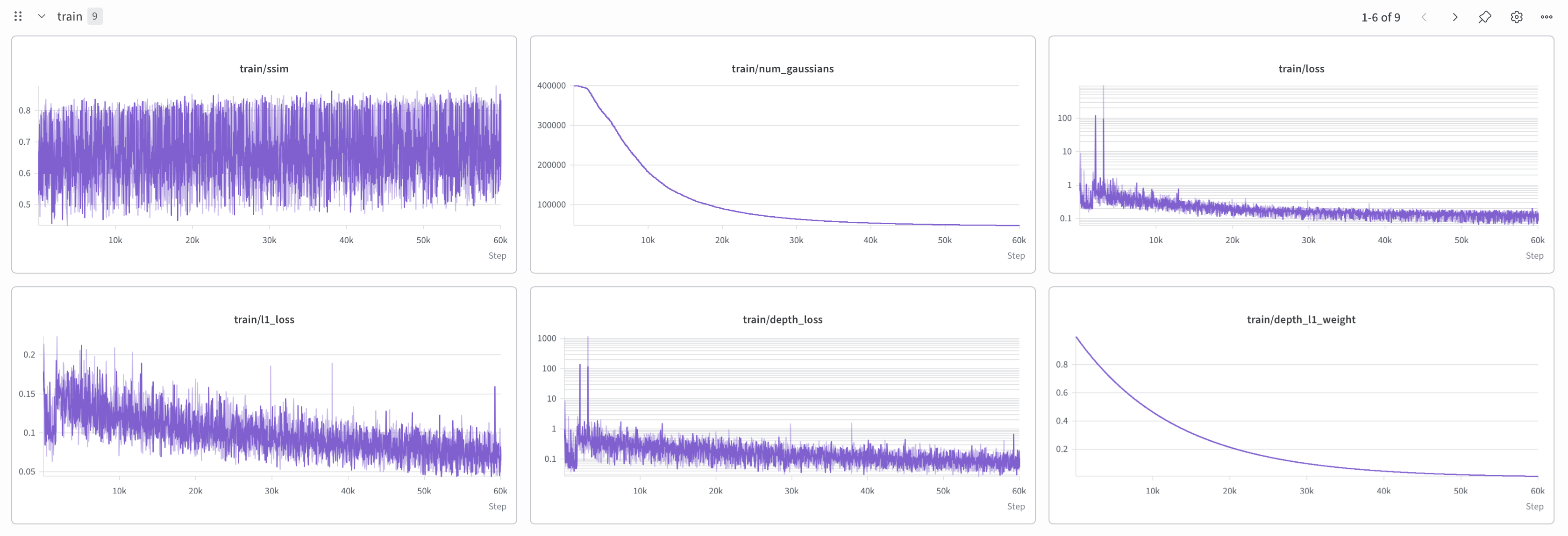
We trained for 60k iterations with densification active for the full run, so that pruning is always paired with clone and split replenishment. Pruning without replenishment collapsed the Gaussian count by about 75%. We completely disabled opacity resets since they produced crystalline artifacts on this scene.

Camera Pose Refinement

This is the single implementation that greatly bettered the structural fidelity of the output.

LoGeR predicts a pose $\pi_k = (R_k, t_k)$ for each frame, with $R_k \in SO(3)$ and $t_k \in \mathbb{R}^3$. Because poses are estimated from local windows, small inter-frame errors accumulate. In the shared 3DGS scene, these errors show up as misalignment, scale inconsistency, and parallax duplicates.

We attached a learnable correction $\delta_k = (\omega_k, \tau_k) \in \mathbb{R}^6$ to each training camera. The corrected pose hence becomes:

\[R'_k = \operatorname{Exp}(\omega_k)\, R_k, \qquad t'_k = \operatorname{Exp}(\omega_k)\, t_k + \tau_k\]

We initialize the correction to $\delta_k = 0$, so optimization starts exactly from LoGeR’s poses. The scene is rendered as $\hat{I}_k = \operatorname{Render}(\Theta, \pi’_k)$ and supervised with the standard L1 + D-SSIM loss $\mathcal{L}_k = \ell(\hat{I}_k, I_k)$. Because the rasterizer is differentiable, gradients reach both the Gaussians and the pose. The two are updated jointly:

\[\begin{aligned} \delta_k &\leftarrow \delta_k - \eta_\delta \nabla_{\delta_k} \mathcal{L}_k \\ \Theta &\leftarrow \Theta - \eta_\Theta \nabla_\Theta \mathcal{L}_k \end{aligned}\]

At each iteration, only the correction for the sampled frame is updated.

Keeping the LoGeR Prior Active

LoGeR’s point cloud is a highly reliable prior for both Gaussian initialization and optimization. We add two terms that keep the prior active even beyond initialization.

Depth Supervision

We took LoGeR’s per-frame camera-space depth and penalize the masked L1 error between rendered and target inverse depth:

\[\mathcal{L}_{\text{depth}}(k) = \frac{1}{|M_k|} \sum_{p \in M_k} \left| \hat{D}_k^{-1}(p) - D_k^{-1}(p) \right|\]

Here $M_k$ is a confidence mask. Its weight decays exponentially from 1.0 to 0.01.

This term only constrains position along the sampled camera’s rays, and it is derived from the same data as the initialization. Alone, it was weak to slightly harmful.

Anchor Loss

Each Gaussian keeps a fixed position $x_g^{(0)}$, which is the point-cloud point it was seeded from. Children created by clone or split inherit their parent’s anchor, so the tether survives densification:

\[\mathcal{L}_{\text{anchor}} = \frac{1}{G}\sum_{g} \lVert x_g - x_g^{(0)} \rVert_2^2\]

Unlike depth, this term is view-independent and constrains all three axes. It catches drift perpendicular to the camera rays, which depth supervision misses.

The two terms are complementary. In a factorial sweep at 60k iterations:

Configuration	SSIM
Anchor loss alone	0.622
Depth supervision alone	0.674
Depth + anchor loss	0.834

Combined, they reached 0.834, the best result overall, with 47,705 Gaussians. The full objective is:

\[\mathcal{L} = 0.8\,\mathcal{L}_1 + 0.2\,\mathcal{L}_{\text{D-SSIM}} + w_{\text{depth}}(s)\,\mathcal{L}_{\text{depth}} + \lambda_{\text{anchor}}\,\mathcal{L}_{\text{anchor}}\]

where $\lambda_{\text{anchor}} = 1.0$.

Relative Extent-Based Threshold Scaling

Replaced scene-extent-dependent densification thresholds, which artificially inflated in large unbounded environments, by anchoring thresholds dynamically to the median point-to-point distance of the initial point cloud.

Results

Which Quantifiable Metrics are Accurate?

The PSNR values in each of our outputs contradicted our visual inspection. Pose correction lowered PSNR by over two points despite producing the largest structural improvement in the output. This is because PSNR rewards per-pixel sharpness from training viewpoints, not consistency across views.

SSIM and photometric loss are most useful when read together. SSIM identifies structural problems well, especially when a scene degrades badly. L1 is noisier, since every step is computed on a different frame, but it catches color and intensity errors that SSIM can miss. When the two parameters disagree, it usually means one aspect of the scene improved at the expense of the other, which is worth checking in the render.

Depth and anchor losses measure agreement with the prior rather than reconstruction quality. Anchor loss tracks drift from initial positions, and depth targets come from LoGeR’s own geometry, so depth loss cannot catch errors in the prior. We can compensate for this in practice. Per-frame depth is locally reliable, and the main source of error, global misalignment between frames, is handled by pose correction.

Structural statistics best predicted specific failure modes. A collapsed maximum Gaussian scale corresponds to sparse, detail-less renders, and a deficit in Gaussian count corresponds to pruned features. The needle-ratio distribution (median 1.55, p99 9.41) further shows that spike artifacts come from a small tail of Gaussians, not the bulk.

Our Final Output

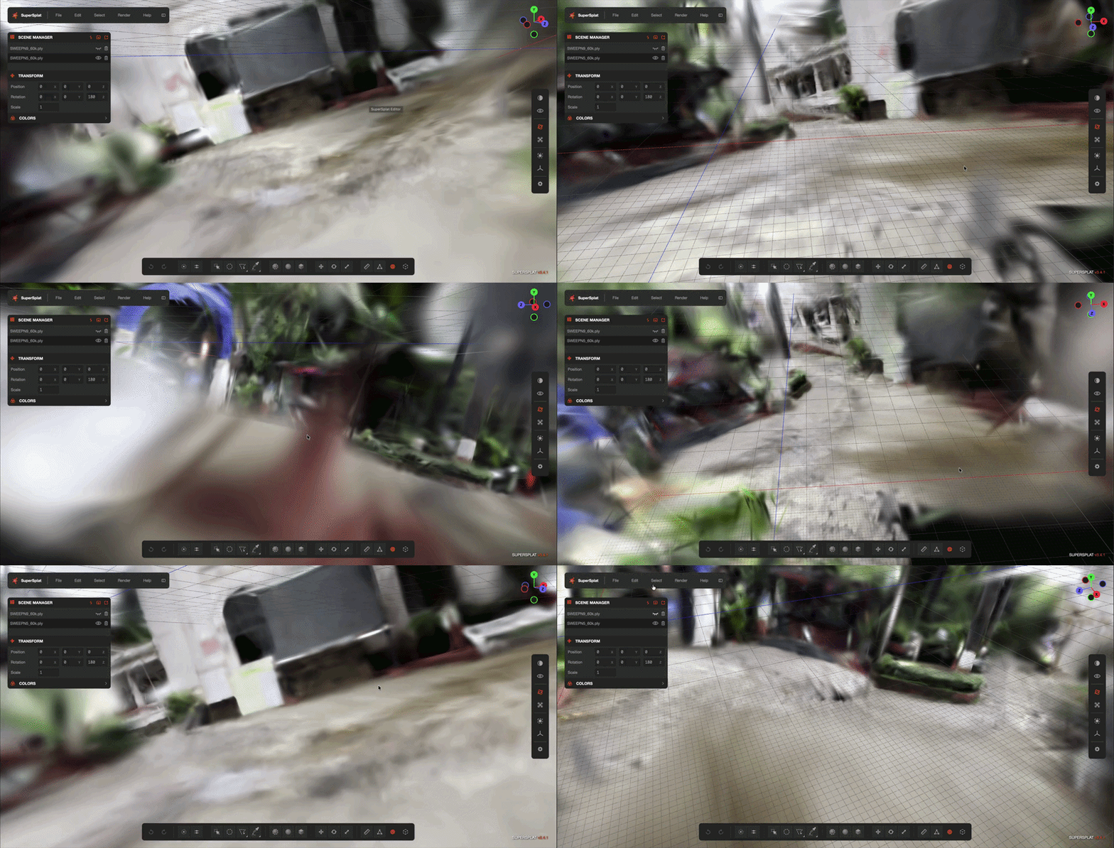
What you see above was trained within 24 GB of VRAM, from a minute-long video taken on a phone camera.

Conclusion

Our biggest realisation was that a strong geometric prior is necessary but far from sufficient. LoGeR’s point cloud gave us a great prior on paper, but with small accumulative inconsistencies, which are definitely hard to avoid when a learned model predicts geometry chunk by chunk over a long sequence, so the downstream optimization has to absorb them. Most of our progress, hence, came from making the optimization respect the prior rather than overwriting it.

The room to improve is still immense, particularly in fine detail. But it’s a good proof of concept that large-scale 3D reconstruction and Gaussian splatting can be both consistent and photorealistic without expensive hardware.

References

1. LoGeR: Long-Context Geometric Reconstruction. https://loger-project.github.io/files/loger_paper.pdf
2. Scal3R: https://arxiv.org/pdf/2604.08542
3. QuerySplat: https://arxiv.org/pdf/2608.01186
4. 3D Gaussian Splatting: https://arxiv.org/pdf/2308.04079
5. Adaptive Voxelization: https://arxiv.org/pdf/2506.00271