24-Karat Magic

• Sarayu Anantharaman
• Shreya Karia
• Vrushtee Gaikwad
• Shashvat Prabhu
• Tirth Gada
• Kushaan Gada

Smart India Hackathon is a national platform where students work on real problems given by government bodies and industries, and actually try to build usable solutions.

We got the chance to participate, cleared two rounds, and made it to the finals at IIT Kharagpur in December of 2025.

The Problem Statement

Our problem statement came from the Bureau of Indian Standards. The goal was to explore new or alternative assaying methods to the traditional fire assay method for testing gold jewellery and artefacts, using non destructive techniques.

Fire assay is accurate but destructive, slow and not suitable when you want to test jewellery without damaging it. BIS is interested in methods that can preserve the artefact while still giving reliable purity and composition data.

What We Tried Before Locking In

Thermal Analysis

The idea: Heat the gold sample to a constant temperature, let it cool, record the cooling using a thermal camera, and plot a cooling curve. In theory, different compositions should cool differently. But in reality, cooling curves depended heavily on size, surface area, volume, and geometry. Two samples of the same purity but different shapes behaved differently. Normalizing for all physical parameters became unrealistic.

Density Measurement

Gold has a density of around 19, while most common impurities sit closer to 8 to 10. This method could roughly separate high purity gold from low purity gold, but that was it. It could not tell what impurities were present or in what proportion.

Computer Vision for Color Detection

Another idea was to use image processing to classify gold based on surface color, such as yellow, white, or rose gold.

The concept relied on converting images from RGB to HSV color space. To reduce variability, we considered designing a controlled imaging environment with fixed lighting conditions, camera parameters, and a standardized sample placement. The idea was to calibrate HSV ranges under this controlled setup and ensure that every test sample would be evaluated under identical conditions.

Even with a controlled environment, the approach remains fundamentally limited. Mixed alloys tend to produce overlapping HSV distributions, making reliable separation difficult. Surface treatments, polishing, plating, oxidation, can significantly alter surface color without reflecting the actual bulk composition. As a result, visually similar HSV values can correspond to very different alloy contents.

The Hallmarking Final Boss

After eliminating other approaches, we landed on Linear Sweep Voltammetry. That’s where things got interesting.

LSV works by linearly increasing voltage over time and measuring the resulting current. When the sample is dissolved in an electrolyte, different metals oxidize at specific voltages. Each oxidation shows up as a peak in current. As voltage increases, metals hit their threshold and start releasing electrons. That release is what we measure as current.

Dissolve the gold sample in an acidic electrolyte like KCl, which produces metal ions in solution. When a metal reaches its oxidation potential, atoms at the electrode surface lose electrons and enter the solution as ions. This produces a graph with different current peaks at different voltages that gives us a clear indication of the composition.

The Math That Makes It Work

LSV produces distinct current peaks as different metals oxidize, but raw peak heights alone do not directly represent composition. Converting these peaks into accurate percentages requires accounting for two fundamental electrochemical effects.

First is electron transfer correction (n-correction). Different metals release different numbers of electrons when they oxidize;

\[\text{Gold: } \text{Au} \rightarrow \text{Au}^{3+} + 3e^-\] \[\text{Silver: } \text{Ag} \rightarrow \text{Ag}^{+} + e^-\] \[\text{Copper: } \text{Cu} \rightarrow \text{Cu}^{2+} + 2e^-\]

Using Faraday’s law, the amount of substance is obtained from the total charge under each peak: $ N = Q /nF$, where $Q$ is the charge (i.e area under the peak), n is the electron transfer number, and $F$ is Faraday’s constant (96,485 C/mol). Without this correction, equal charge would incorrectly imply equal metal content, violating basic electrochemistry.

The second correction accounts for diffusion effects in the electrolyte. In 0.1M KCl, different metal ions diffuse at different rates. Gold forms a bulky AuCl₄⁻ complex that diffuses more slowly than ${Ag}^{+}$ or ${Cu}^{2+}$, which suppresses its current response and makes gold appear less abundant than it actually is. Electrochemical theory shows that current scales with the square root of the diffusion coefficient, so we apply a metal-specific diffusion normalization factor proportional to $√D$ to correct for this transport limitation. Together, electron transfer correction and diffusion normalization convert raw voltammetric peaks into chemically meaningful composition data. Skipping either step can shift calculated purity by tens of percent, which is unacceptable for hallmarking.

With the corrected mole value and the molar mass value we can find individual masses for each element detected and can hence find the percentage mass of each impurity.

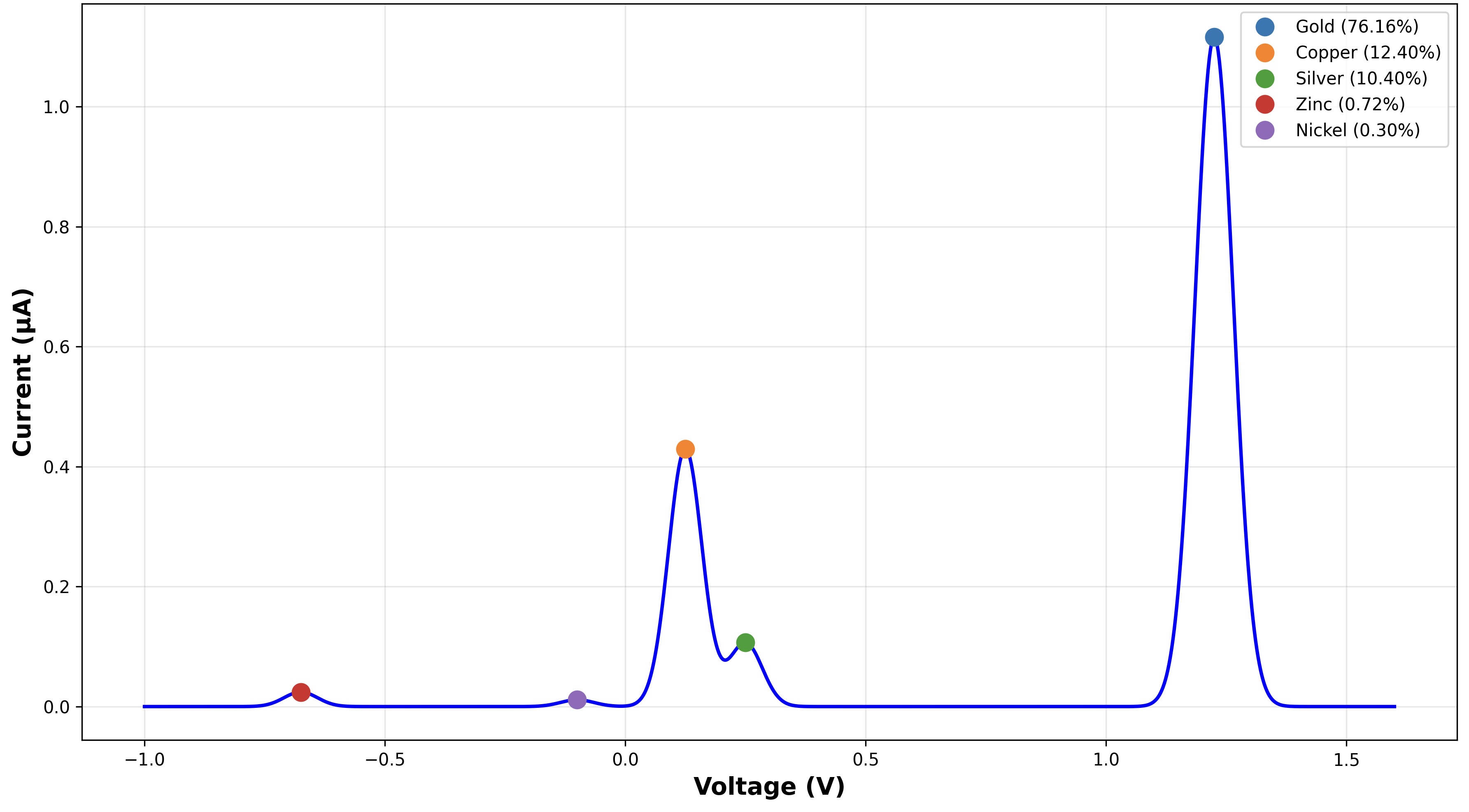
Reading the Graph

The readings give a plot of current versus voltage. Each peak in current corresponds to a metal. The voltage position tells you which metal it is.

Area under the curve of the peak tells us how much of the metal is present.

This lets us detect gold and common impurities like copper, silver, and platinum in a single scan.

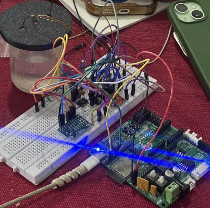
The Circuit

This circuit is a small potentiostat-style, that does one job: sweep the cell’s bias and record how much current the sample draws at each step, so you can plot a clean LSV curve and compare alloys by their electrochemical “fingerprint”.

Input: a programmed sweep (the bias you command), the electrochemical cell (WE/RE/CE), and stable 3.3 V power.

Output: commanded bias → measured current

Control Flow

1. Firmware generates a step-by-step sweep (commanded bias/potential) and outputs it via the DAC/bias control.
2. The cell sees that bias around mid‑rail, so the analog stages can represent the response on a single 3.3 V supply.
3. Cell current is converted to a voltage by the TIA using 50 kΩ effective feedback (we had two 100 kΩ in parallel).
4. ADS1115 samples that voltage and firmware converts it into an estimated current (and marks saturation/clipping if it hits limits).
5. What you display at the end is a plot/table of current vs commanded bias/potential (LSV curve), optionally with the raw ADC values and saturation flags for debugging.

Why mid‑rail + ADS1115 + 50 kΩ makes sense

1. The Virtual Ground: keeps the measurement centered so you don’t instantly rail when the current changes sign; it’s the simplest way to do bipolar-looking measurements on a single supply.
2. ADS1115 powered by 3.3 V: improves readability and repeatability of small signal changes; you’re not fighting noisy, low-resolution readings.
3. 50 kΩ TIA gain: a deliberate middle ground that is high enough to see microamp-scale changes, low enough to avoid saturating constantly when the chemistry pulls more current.

What “good data” means in this setup

1. The curve is trustworthy when the measurement stays away from rail and the run is repeatable across sweeps.
2. When the system saturates (ADC clipping or analog output limiting), those points are still logged but should be treated as “out of range” rather than real chemistry.

Why LSV Should Work

1. detects multiple metals at once
2. needs very small sample volumes
3. fast compared to traditional methods
4. gives quantitative results instead of just classification

Hardware Execution Gaps

Reference electrode instability: Bare copper wire drifted ±50-200mV during scans. Professional systems use Ag/AgCl electrodes with saturated KCl buffers (±1mV stability).

Wrong voltage window: Scanned 0-1.8V when gold oxidation peaks occur at 0.1-0.5V. Above 0.6V, water electrolysis dominated (>1µA background), masking the metal signals we needed.

ADC misconfiguration: Gain set to ±0.256V range while circuit output 0-3.3V, producing negative readings and unreliable current calculations.

Lab-grade LSV requires platinum working electrodes (₹15,000+), buffered reference electrodes with salt bridges (₹8,000+), temperature control (±0.1°C), nitrogen purging to remove dissolved oxygen, and reagent-grade electrolytes. We had copper wires in unbuffered KCl at room temperature with ambient oxygen.

Small variables compound into large errors. Fingerprint oil changes peak heights. Stirring rate affects diffusion. Scan speed distorts peaks. Without these controls, identical samples produced peaks varying 40-60% when hallmarking requires ±5% tolerance.

The Outcome

By the end of five days, we had:

1. Established a functional proof-of-concept for using LSV for gold hallmarking
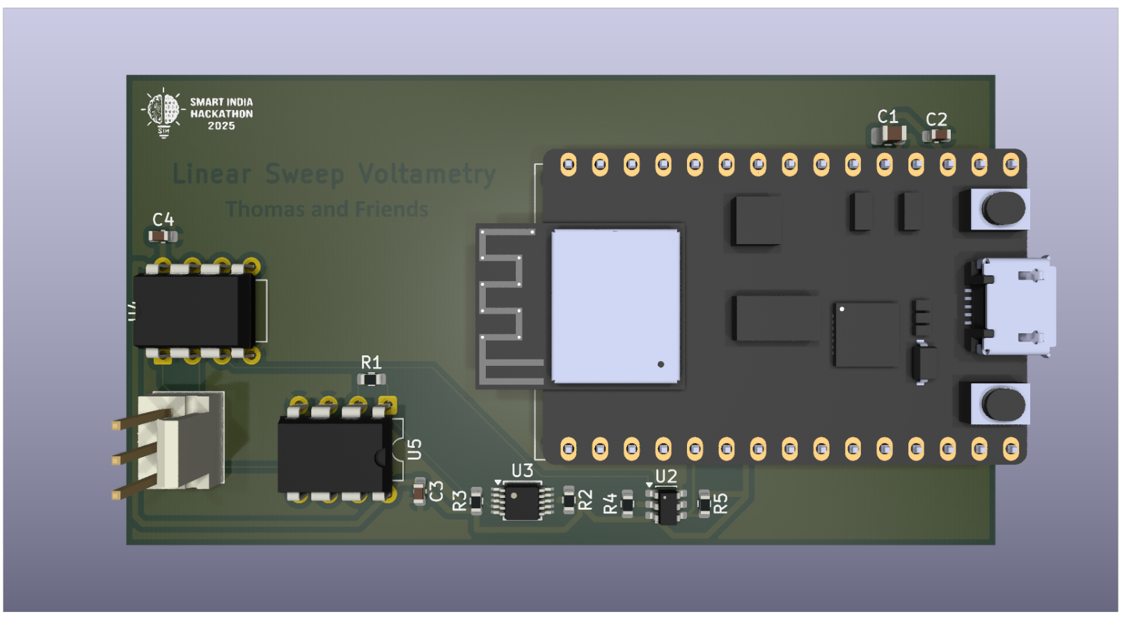
2. Designed and simulated a PCB for the LSV circuitry
3. Validated the overall electrochemical approach, with limitations mainly in execution and integration rather than theory.

In the context of the problem:

1. No team could arrive at a complete end-to-end solution
2. The judges noted the difficulty of the problem and shared that approaches like ours would require significantly more time to deploy

Why This Problem is Hard

Fire assay works because it’s purely thermal—robust to sample prep, geometry, and technique. Electrochemical methods are sensitive to surface condition, solution chemistry, temperature, and kinetics in ways that make field deployment challenging.

A jeweler-usable instrument needs automated surface prep, sealed multi-year reference electrodes, temperature compensation, and calibration databases mapping peaks to compositions.

The science is sound: In five days of experimentation, we achieved developing a viable proof of concept around the physics of it. What remains now is disciplined and iterative engineering.