Through Feature Matchers

– Prajwal Avhad

The process of matchers has always been broken down into two key steps, a pattern that will define every architecture

• Feature Detection: First, find interesting and reliable points in an image.
• Feature Description: Then, for each of those points, create a unique fingerprint.

SIFT and SURF were incredibly robust, producing high-quality results that set the standard for accuracy. In 2011, a paper was published that changed the landscape. It introduced ORB, the proposed ORB = Oriented FAST + Rotated BRIEF.

---

• FAST produced low-quality, non-oriented corners.
• BRIEF’s descriptors were not rotation-invariant.

This is the core of their paper, adding orientation to FAST and make BRIEF rotation-invariant.

---

Section 1 - ORB

oFAST: FAST Keypoint Orientation

The first task was to upgrade the FAST corner detector. The authors addressed its two main weaknesses: its tendency to find many low-quality points and its lack of orientation.

Finding Better Corners

Instead of just taking every corner FAST finds, oFAST uses a multi-step quality control process:

1. First, run FAST with a low threshold to detect a huge number of potential keypoints.
2. Then, use a Harris corner measure to score each of these points for quality. This removes unstable points found along edges.
3. Sort the points by their Harris score and pick only the top N best corners.
4. Repeat this process over an image pyramid (a stack of downscaled versions of the image) to make sure that both large and small corners are found.

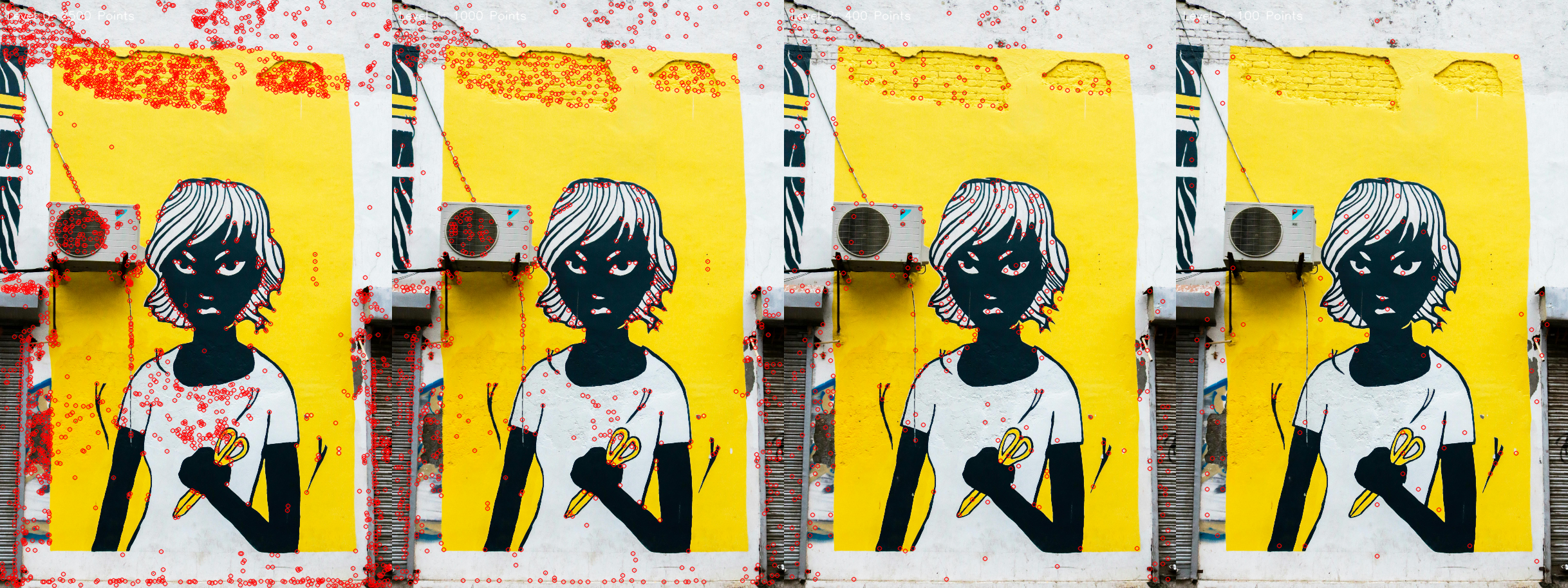Detecting features across multiple scales ensures robustness to distance.

Orientation by Intensity Centroid

With high-quality corners in hand, the next step is to give them an orientation. ORB does this with a beautifully simple method: the intensity centroid.

For a patch of pixels around a keypoint, this method calculates its center of mass, where the mass of each pixel is its brightness. The orientation $\theta$ is then defined as the vector pointing from the corner’s center to this intensity centroid.

\[\theta = \text{atan2}(m_{01},m_{10})\]

Here, $m_{01}$ and $m_{10}$ are the moments that represent the total intensity distribution along the $y$ and $x$ axes, respectively. With this, every keypoint now has a reliable orientation.

Results -

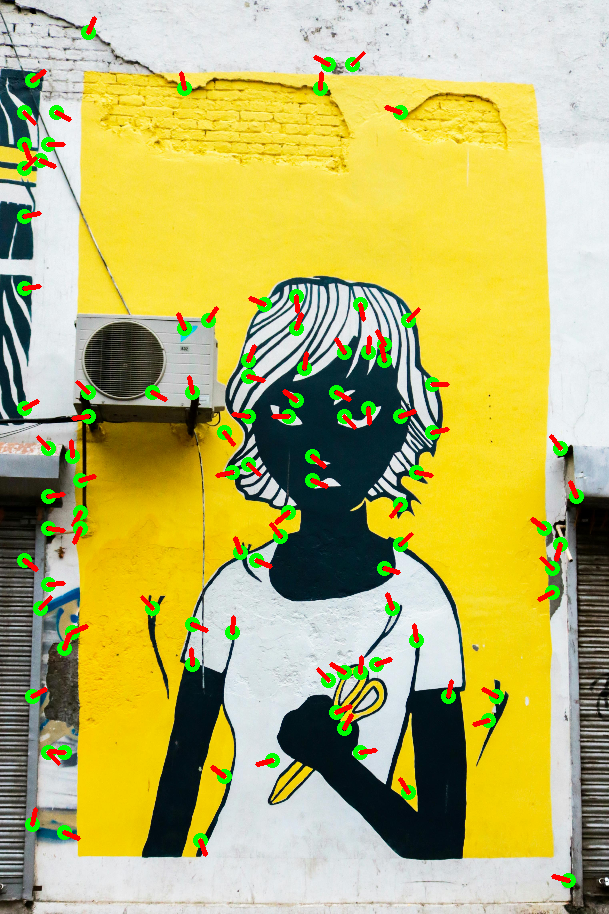
The green circles being the corner and red arrows showing their orientation.

---

rBRIEF: Rotation-Aware Brief

Let us take a look at BRIEF descriptor in short.

First you detect keypoints, usually using FAST, BRIEF will only describe these points. For each keypoint extract a image patch, here 31x31.

BRIEF defines a set of $n$ pairs of points within the patch. ($n$ = 256)

\[\tau(\mathbf{p}; \mathbf{x}, \mathbf{y}) := \begin{cases} 1 & :\ \mathbf{p}(\mathbf{x}) < \mathbf{p}(\mathbf{y}) \\ 0 & :\ \mathbf{p}(\mathbf{x}) \geq \mathbf{p}(\mathbf{y}) \end{cases}\]

The problem, as shown below, is that if the image rotates, the random pattern of pixel pairs also rotates, leading to a completely different binary string.

Original BRIEF fails when the image is rotated.

The obvious solution is to “steer” the BRIEF pattern: take the orientation $\theta$ we just calculated with oFAST and rotate the 256 test-pairs accordingly before comparing pixels. Simple, right?

Well, it didn’t work. The authors found this intuitive “Steered BRIEF” actually performed worse than the original.

This led to a crucial insight: a good set of binary tests needs two properties:

1. High Variance: The bits should flip between 0 and 1 often. A bit that is always 0 provides no information.
2. Low Correlation: The bits should be independent. If two bits always flip together, one of them is redundant.

The original BRIEF pattern, when arbitrarily rotated, lost these properties. The test pairs became correlated. So, the authors used a machine learning approach. They ran a greedy search on a huge training set of image patches, analyzing thousands of possible pixel pairs. Their goal was to find a new, optimized set of 256 pairs that, even after being rotated, would remain highly variant and uncorrelated.

This new, learned set of tests is what we call rBRIEF.

rBRIEF, using a learned pattern, is robust to rotation.

So this was the concept of ORB, fun little feature descriptor.

Section 2 - The Rise of Learning

ORB was, and still is, a brilliant piece of engineering. It’s fast, and for many applications, it’s good enough. But as the demands of SLAM, 3D reconstruction, and image matching have grown, the classic approach of ORB is starting to go down. Before we jump into its successor, let’s look at why the community started searching for something better, referencing the SuperPoint.

1. ORB is great at finding corners, but it often finds too many in the most textured parts of an image. As the SuperPoint paper notes, “the detections cluster together.” This leaves large, less-textured areas of the image completely bare, which isn’t ideal if the camera moves to view those areas.
2. This point clustering means that while you might have high repeatability.

Section 3 - SuperPoint: Self-Supervised Features

SuperPoint, like ORB, aims to find interest points and their descriptors. But instead of using hand-crafted rules, it uses a deep convolutional neural network.

---

How do you train a neural network to find interest points? You need a massive dataset with ground-truth labels. But what is a perfect ground-truth interest point? The goal is to create a huge, high-quality dataset of interest points on real images without any human labeling.

---

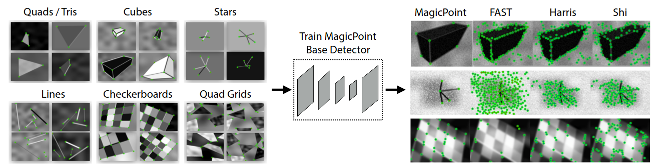
Step 1: Start with Fake Data (MagicPoint) -

First, they generate a large dataset of simple synthetic shapes: squares, triangles, stars, etc. (They call this Synthetic Shapes). For these shapes, the corners are perfectly known. They train an initial, basic detector on this fake data and call it MagicPoint. It’s good at finding corners on simple shapes but not great on complex, real-world images.

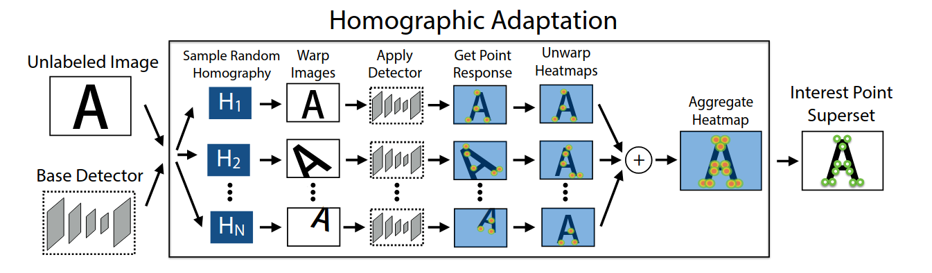
Step 2: Homographic Adaptation -

They take a real, unlabeled image from a dataset like MS-COCO.

• Warp this image hundreds of times with random homographies (rotating, skewing, changing perspective).
• Run their basic MagicPoint detector on each of these warped images.
• Then, “un-warp” all the detected points back onto the original, un-warped image.
• The points that were consistently detected across many different warps must be the most stable points. These points that survive the distortion become the “pseudo-ground truth” labels.

This process, called Homographic Adaptation, it lets the model teach itself what a good, robust corner looks like on real images.

Step 3: Train the Final Network (SuperPoint) -

Now, with this massive new dataset of real images and self-generated labels, they train the final, powerful SuperPoint network. This network is a single, unified model that takes a full-sized image and, in one forward pass, outputs both the interest point locations and their descriptors. This is more efficient than ORB’s separate detect then describe pipeline.

Section 4 - SuperGlue

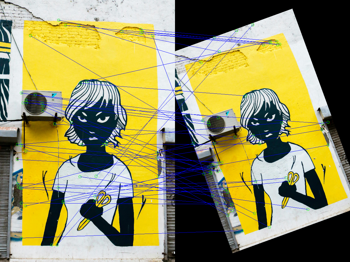
With ORB, we use a simple brute-force search: take a descriptor from image A and find the one in image B with the smallest distance (e.g., Hamming distance). This is called nearest neighbor matching. It’s fast, but it’s naive. It less feature environment it fails.

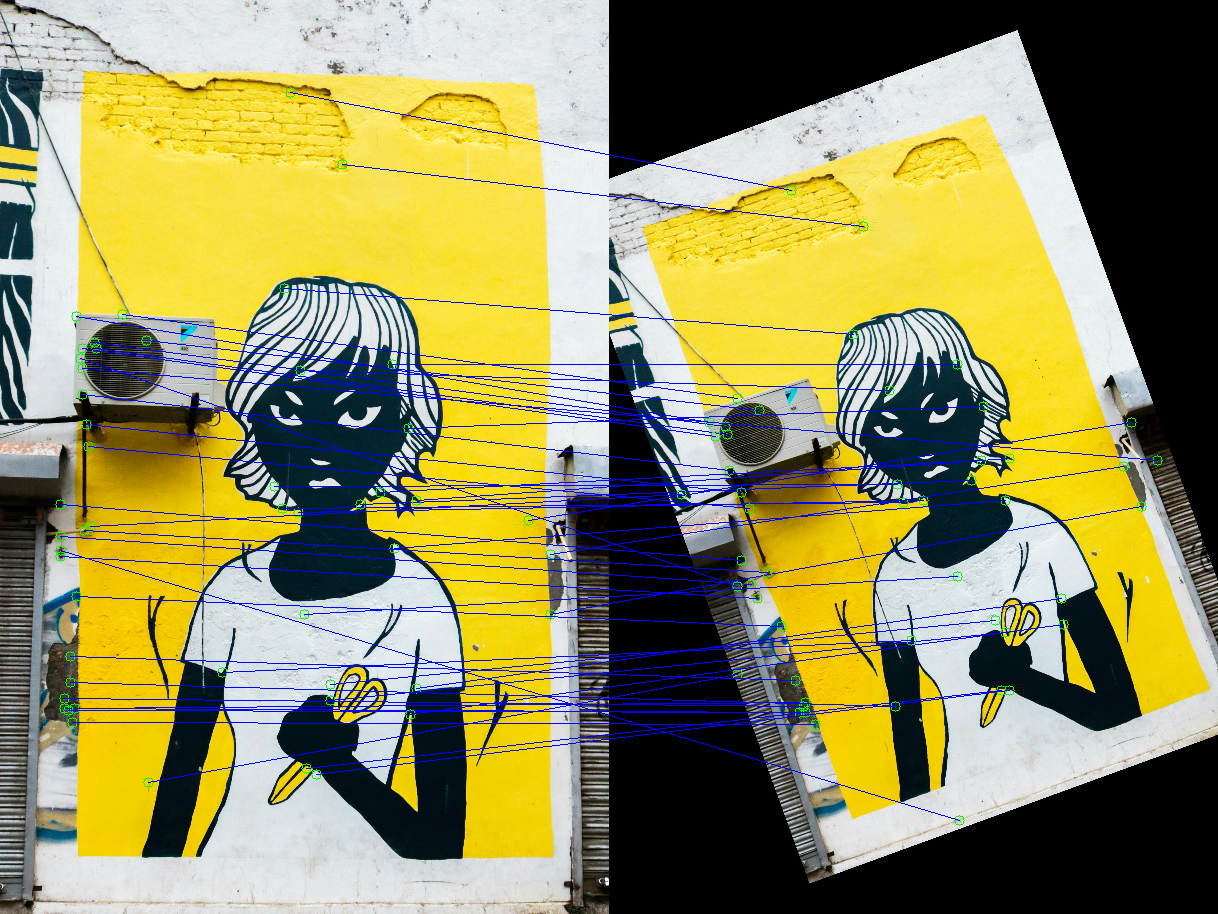
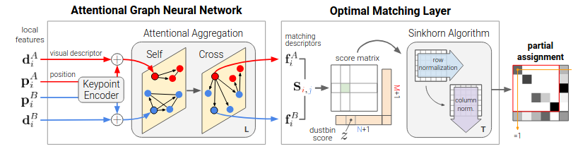
SuperGlue is not a feature detector, it’s a dedicated matcher. It takes the keypoints and descriptors from two images (like those from SuperPoint) and, figures out which ones correspond. It uses something known as Attentional Graph Neural Network.

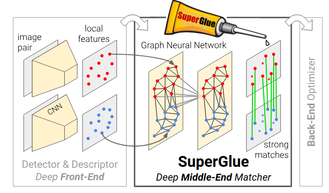
Keypoint encoder -

Before the attention mechanism can start, SuperGlue needs to combine a keypoint’s visual appearance with its location. It can’t just look at the descriptor, it also needs to know where the point is. It does this with a Keypoint Encoder.

For each keypoint $i$ in an image, we have its visual descriptor $d_i$ (from SuperPoint) and its position $p_i = (x, y)$. The encoder uses a simple Multilayer Perceptron (MLP) to transform the position into a high-dimensional vector and adds it to the descriptor. This creates the initial “context” vector $x_i$

\[\ ^{(0)} \mathbf{x}_i = \mathbf{d}_i + \mathrm{MLP}_{\mathrm{enc}}(\mathbf{p}_i)\]

This initial vector $^{(0)}x_i$ now contains both visual and spatial information.

Self and Cross-Attention Layers -

The model iteratively refines these initial vectors $x_i$ by letting them communicate with each other. It does this using alternating layers of Self-Attention and Cross-Attention.

The core mechanism is the same for both, based on the classic query-key-value attention model from Transformers:

1. Query (q): “What am I, as a keypoint, looking for?”
2. Key (k): “What am I, as another keypoint, able to be found by?”
3. Value (v): “If I am found, what information should I share?”

For a given keypoint $i$, it calculates an attention weight $\alpha_{ij}$ for every other keypoint $j$. This weight is essentially the similarity between $i$’s query and $j$’s key. The higher the similarity, the more “attention” $i$ pays to $j$.

\[\alpha_{ij} = \mathrm{Softmax}_j(\mathbf{q}_i^\top \mathbf{k}_j)\]

Once it has these weights, it computes a “message” m by taking a weighted sum of all the other points’ values. Basically, it aggregates information from all other points, but it listens more closely to the ones it pays more attention to.

\[\mathbf{m}_i = \sum_j \alpha_{ij} \mathbf{v}_j\]

This message $m_i$ is then used to update the keypoint’s vector $x_i$, creating a new, more context-rich vector for the next layer. This is repeated for L layers.

Now, here’s how this applies to our two steps:

• Self-Attention Layers: The communication happens within the same image. Keypoint $i$ in image $A$ communicates with all other keypoints $j$ also in image $A$. This builds a good understanding of the scene’s internal structure.
• Cross-Attention Layers: The communication happens between the two images. Keypoint $i$ in image $A$ communicates with all keypoints $j$ in image $B$. This is where it actively searches for potential matches, guided by the context it built during self-attention.

SuperGlue alternates between these layers (Self → Cross → Self → Cross…), allowing information to flow both within and between the images, actively refining the feature representations until they are robust and context-aware.

Matching Layer -

After L attention layers, we have a final, powerful set of feature vectors, let’s call them $f_i^A$ for image $A$ and $f_j^B$ for image $B$. Now we need to make the final assignments.

First, SuperGlue computes a score matrix $S$, where each entry $S_{ij}$ represents the matching likelihood between point $i$ from $A$ and point $j$ from $B$. This is simply the dot product of their final feature vectors:

\[S_{ij} = \langle \mathbf{f}_i^A, \mathbf{f}_j^B \rangle\]

A simple approach would be to pick the highest score for each row and column, but this can lead to conflicts. Instead, SuperGlue solves this as a linear assignment problem. It uses a differentiable algorithm called Sinkhorn.

The Sinkhorn algorithm takes the entire score matrix S and finds the optimal partial assignment that maximizes the total score, while having two constraints:

• A keypoint can be matched to at most one other keypoint.
• Some may not be matched at all (due to occlusion or leaving the frame). These are basically ignored.

Problem?

This incredible reasoning power comes at a cost. The attention mechanism, especially when considering all possible pairs, is computationally very heavy. While the paper shows it running in real-time on a modern GPU, SuperGlue is heavyweight.

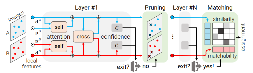
Section 5 - LightGlue

How I see it is LightGlue = Lightning Fast SuperGlue

LightGlue’s efficiency comes from fundamentally changing how it encodes positions, how it makes decisions, and how it manages the computation itself.

SuperGlue used an absolute positional encoding, adding a vector based on a keypoint’s $(x, y)$ coordinates. The LightGlue authors suggesst that this information tends to get forgotten in deeper layers. They replaced it with a relative positional encoding (specifically, Rotary Encoding) that is only used during self-attention.

In self-attention, when point $i$ calculates its attention to point $j$, the score is now a function of their relative position $(p_j - p_i)$.

\[\alpha_{ij} \propto \mathbf{q}_i^\top R(\mathbf{p}_j - \mathbf{p}_i) \mathbf{k}_j\]

Here, $R()$ is a rotation matrix that rotates the key vector $k_j$ based on the relative position $(p_j - p_i)$.

This is a major change. SuperGlue used the powerful but expensive Sinkhorn algorithm to solve the assignment problem. LightGlue replaces it with a much lighter two-part head that is faster and easier to train.

For each potential match $(i, j)$, LightGlue predicts two things:

1. Similarity Score ($S_{ij}$): How well do the final feature vectors of $i$ and $j$ match? This is a simple linear projection and dot product.
2. Matchability ($\sigma_i$): How likely is point $i$ to be matchable at all? A point that is occluded or looking at a textureless sky should have a low matchability. This is learned with a simple Sigmoid classifier.

\[\sigma_i = \mathrm{Sigmoid}(\mathrm{Linear}(\mathbf{x}_i))\]

The final assignment matrix $P$ is then calculated by combining these two scores using a double-softmax , which acts as a fast substitute for mutual nearest-neighbor checks.

\[P_{ij} = \sigma_i^A \sigma_j^B \cdot \mathrm{Softmax}_k(S_{ik}) \cdot \mathrm{Softmax}_k(S_{kj})\]

Hence, LightGlue can adapt the amount of computation based on the difficulty of the image pair.

Adaptive Depth: After each Transformer layer, a small confidence classifier predicts if a point’s representation is final. If a high percentage of points are confident, the network simply stops and outputs the current matches. For an easy pair of images (like two sequential video frames), it might exit after only 3 of 9 layers, saving immense computation.

\[\text{exit if} \left( \frac{1}{N+M} \sum_{I \in \{A,B\}} \sum_{i \in I}[c_i > \lambda_c] \right) > \alpha\]

Adaptive Width: As the layers progress, LightGlue identifies points that are confidently unmatchable (suppose in areas with no visual overlap). It then prunes these points, removing them entirely from the attention mechanism in subsequent layers. Since the complexity of attention is quadratic with the number of points, this provides a massive speedup on difficult image pairs with low overlap.

Finally, we arrived at the current state-of-the-art. LightGlue refined the powerful ideas of SuperGlue, making them adaptive, efficient, and blazing fast.

So yeah that’s a very “brief” history of feature matchers. Thank you for reading!!

In the next few blogs I’ll try my best to summarise the architecture of visual SLAM, and break it down. Feature matching is one of its key building blocks, more on that soon….