Exploring the magic of RL,making machines learn!!!!!

Mentees:

– Ansh Semwal

– Gaurav Tatpate

– Vyoma

GYM - MASTER :

What is our project?

Our project pushes us to explore the uncharted waters of RL - REINFORCEMENT LEARNING. Building a solid foundation on key concepts of RL, learning the relevant and necessary technologies of PyTorch and/or TensorFlow. We then implement our learnings to solve various OpenAI gym environments and then move on to make a marquee project utilising all our learnings.

Intro to RL

This is where we discuss the very fundamentals of RL. So what exactly is RL?

Reinforcement learning is the multi-disciplinary area of machine learning where an intelligent agent is made to learn about its dynamic environment by interacting with it and then to maximize a reward function to ultimately solve a problem.

So how does it work?

Well, basically you send in your bot/agent into the environment (anything that your agent cannot control is the environment) and it gets to tinkering, i.e., giving the environment some input. The environment takes this input, processes it, makes the necessary changes in itself as directed by the input, and spits out an output for the agent. This is then taken by the agent as an input for itself. This output by the environment is called a reward, a measure of how good or bad our agent’s decision is. And we do all of it again.

Through these continuous steps, we create and then update the value function for all the actions and states. This value of a state or action is the total amount of reward an agent can expect to accumulate over the future, starting from that state or action.

Besides this, we also learned some basic definitions of various components of a standard RL model, which are provided in further sections. Just know that we were armed with basics of RL, some Python, and some Numpy magic. Now onto solving our very first problem.

K-armed Bandit :

K-armed bandit problems, where the agent chooses from a large number of levers or actions. Each of these actions yields the agent a reward. The task is then to maximize this reward that the agent receives. The value of any action ( a ) taken at time-step “t” then is:

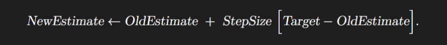
where ( R(t) ) is the reward for that time-step. We do not have the value of all the actions, we need to estimate this value to make decisions, which we do by taking averages of rewards .But we also have to update this value for each time-step which we do using this formula:

Exploitation vs exploration

• Exploitation: The action of repeatedly choosing the action that yields max reward (also called greedy action) is called exploitation.
• Exploration: The action of choosing a variety of different actions (non-greedy actions) and not exclusively choosing one is exploration.

Agent has to exploit what it has already experienced,but it also has to explore in order to make better action selections in the future. The dilemma is that neither exploration nor exploitation can be pursued exclusively without failing at the task. The agent must try a variety of actions and progressively favor those that appear to be best. This dilemma is unique to reinforcement learning.

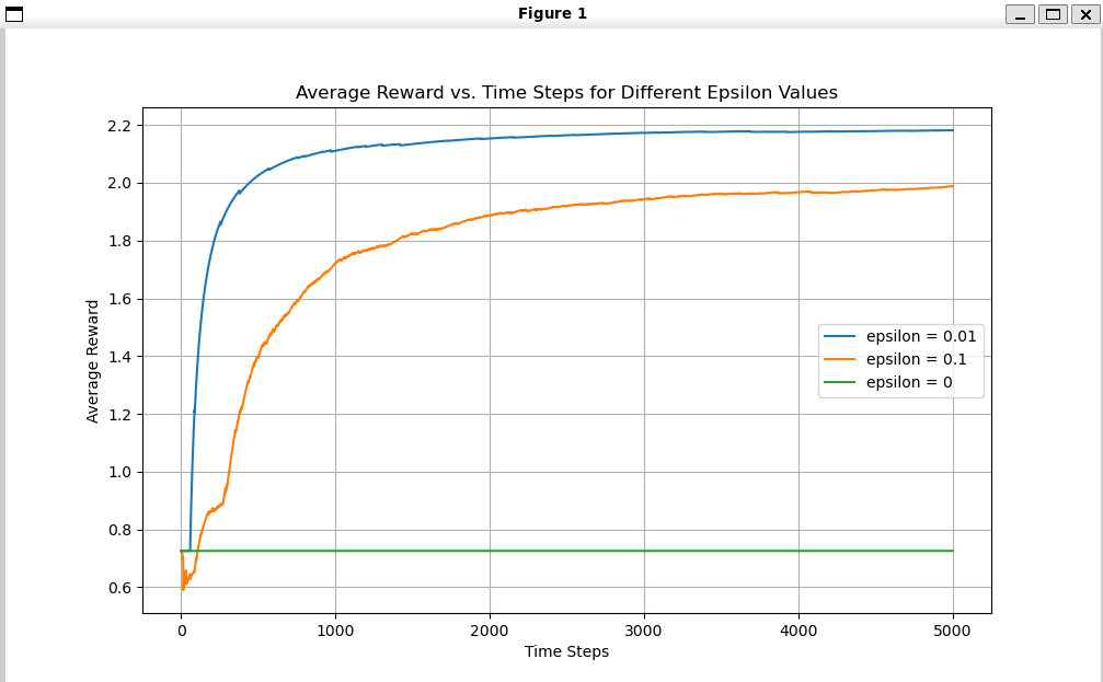
To solve this, we use a strategy called the epsilon-greedy strategy. The idea is to spam greedy action with a mix of non-greedy action in between. The non-greedy action will be executed with the probability of epsilon (a small number generally 10%) and the greedy action will be taken up with the probability of 1-epsilon. By this, we are able to find a middle ground between the two extremes.

Markov decision process (MDP)

Introduction

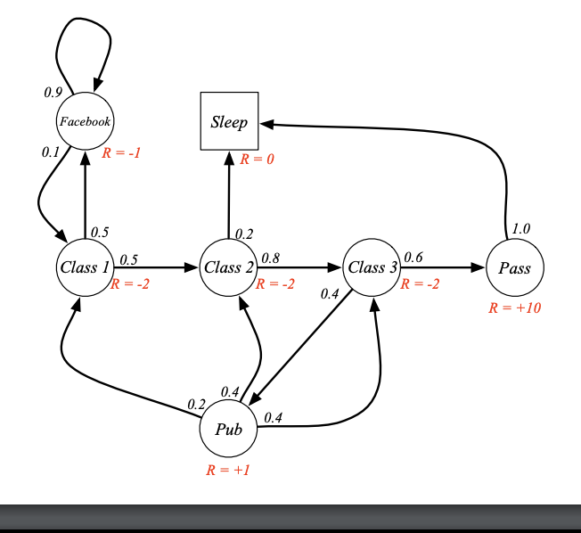
Markov Decision Processes (MDPs) provide a mathematical framework for modeling decision-making. Here we work with the Bellman equation and its forms to find the next actions and assign values to the states. MDPs are essential in fields like artificial intelligence and reinforcement learning.

A Markov state follows the property:

This means that “the future is independent of the past given the present”.

Key Concepts

1. Transition Probabilities: These probabilities indicate the likelihood of moving from one state to another, given a specific action. For example, what is the probability of a piece moving from D3 to B5?

2. Policies: A policy is a strategy that defines the action to be taken in each state. In chess, a policy could be a strategy that tells you which move to make in each configuration of pieces.

3. Value Function: The value function measures the expected return (total rewards) starting from a state and following a particular policy. For example, the expected points you would get from a certain state in the game if you follow a particular strategy. We calculate the value function using the Bellman Equation which is:

   

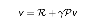
4. Discount Factor: The discount factor is a value between 0 and 1 that reduces the value of future rewards to account for uncertainty and delay. This means preferring an immediate reward over a future one because the future is uncertain.

Conclusion

Markov Decision Processes form the backbone of many reinforcement learning algorithms by providing a structured way to handle decision-making under uncertainty. By understanding states, actions, rewards, and policies, we can design intelligent systems capable of making optimal decisions over time.

Dynamic Programming

Introduction

Dynamic programming is a mathematical way of mapping states to actions and then maximizing the policy of doing so. It refers to a collection of algorithms that can be used to compute the optimal policy given that there is a perfect model of the environment, such as an MDP. It breaks down problems into subproblems, and then the optimal solution to the subproblems helps you find the optimal solution to the main problem.

Key Concepts Involved

• Policy: It tells us the actions that we have to take based on our current state.
• Value Function: It tells us the expected return of a function following a policy from that state onwards.
• Action Value Function: It tells us the expected return starting from state (s), following action (a) and following a particular policy.

Uses of Dynamic Programming

• Used to plan an MDP:
  • Prediction:
    • Input: Tells us the MDP.
    • Information such as the state, probability, and gamma are given.
    • The output is a value function.
    • We have to calculate the best possible reward from the already given policy.
  • Control:
    • MDP is given, i.e., all parameters are given.
    • The output is the optimal value function.
    • We evaluate policies and improve them iteratively to get maximum rewards.

Algorithms

• Prediction: Policy Evaluation
  • Steps:
    1. Initialize the state of the value function to an initial value.
    2. Set a threshold for convergence.
    3. Update the value function according to the Bellman expectation equation.
    4. If the final value is smaller than the value of the threshold, then we stop the iterations.
• Control: Policy Improvement
  • Steps:
    1. The policy and initial value function will be given.
    2. Using the current value function, we compute the action value function for state and action.
    3. We improve the policy by making it greedy with respect to the action value function.
    4. We basically have to choose an appropriate action to maximize the action value function.
    5. We compare the updated policy with the previous policy, and if it is the same as the previous, then it is said to be stabilized and to be the optimal policy.
• Policy Iteration
  • It combines policy evaluation and policy improvement and runs it in a loop.
• Value Iteration
  • Initialize a value function.
  • Update the value function using the Bellman Optimality equation.
  • Stop when the change is smaller than the threshold for convergence.
  • Once the value function has converged, obtain the optimal policy by choosing the action that maximizes the action value function in the policy.

Grid World Problem Overview

The grid world problem is a simple game used to teach basic ideas in reinforcement learning. In this game, an agent (like a robot) moves around a grid, aiming to reach a goal while avoiding dangerous spots.

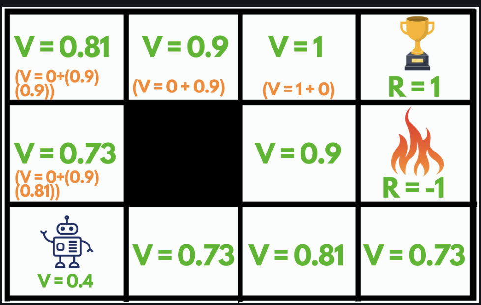
Setup

• Grid: A 4x4 grid where each cell is a different state.
• States:
• Winning State: Reaching this cell gives a reward of +1.
• Losing State: Reaching this cell gives a penalty of -1
• Neutral State: All other cells have no reward (0).
• Actions: The agent can move:
  • Up
  • Down
  • Left
  • Right

Our Solution: Value Iteration

To solve this problem, we use a method called value iteration. This method helps the agent learn the best way to move to reach the goal while avoiding danger.

Steps

• Initialize: Start with all values set to 0.
• Iterate: Update the values of each state by looking at possible actions.
• Calculate Value: For each action, calculate the expected reward and update the value of the state.
• The process continues until the change in the value function is less than a small threshold (theta), indicating convergence.
• Determine Policy: Find the best action for each state based on the calculated values.\

What have we done till now?

These past weeks we have laid the foundation for our journey ahead. Taking the time to learn the basics of RL and then subsequently apply them on various OpenAI-GYM environments has been our primary concern.

What are we referring to?

Since the last 3 weeks we’ve been going through a video lecture series on RL by Prof. David Silver uploaded on Google DeepMind’s official YouTube channel. Along with this, we’ve been referring to Reinforcement Learning: An Introduction, authored by Richard Sutton and Andrew Barto, and many other videos across the internet.