 The Society of Robotics and Automation is a society for VJTI students. As the name suggests, we deal with Robotics, Machine Vision and Automation
Moving ahead with the project - Rotary Inverted Pendulum
Following an introduction with the basics of Rotary Inverted Pendulum, we have now entered the simulation phase of our project. So we are using MATLAB as our simulation software. We simulated systems like Simple pendulum and Spring mass system. For this, we first derived the Lagrangian equations for these.
What are Lagrangian equations?
The Lagrangian function is a quantity that characterises the state of a system. The Lagrangian L is defined as L = T − V, where T is the Kinetic energy and V the Potential energy of the system in question. Generally speaking, the potential energy of a system depends on the coordinates of all its particles; this may be written as V = V(x 1, y 1, z 1, x 2, y 2, z 2, . . . ). The kinetic energy generally depends on the velocities, which, using the notation v x = dx/dt = ẋ, may be written T = T(ẋ 1, ẏ 1, ż 1, ẋ 2, ẏ 2, ż 2, . . . ).
What is Simulation?
Well, a simulation is the imitation of the operation of a real-world process or system over time. simulation represents the evolution of the model over time In the process, we were introduced to MATLAB. Understanding the Syntax of Matlab is certainly the most complex step till now. We got to understand functions like “Ode”, ‘Draw’, ‘Rectangle’. Custom functions were formed in order to achieve desired outputs. We were required to even animate the systems for which we used function like rectangle and line where in we could form a rectangle and give it a curvature as that of a bob in case of a simple pendulum. This has certainly opened a new dimension in our technical knowledge and we are excited and thrilled to move forward with our Eklavya Project.
Simulation in Ideal state as well as using the concept of LQR (Linear Quadratic Regulator)
We consider any system to be of the form ẋ = Ax + Bu where x is the state vector and u is the external input provided. In an ideal system we do not provide any external input u.
Simulation of an ideal pendulum system : Initial point: -pi/3 ideal_pendulum
Simulation of an ideal spring-mass system: Initial point: (1,0) ideal_spring
Using LQR: LQR is basically used to control the system. In the case of a system of a pendulum, we define a setpoint along with the initial point which is actually the point where the pendulum is stable as in this case. For this, we also define a cost function.
What is a cost function?
The cost function is often defined as a sum of the deviations of key measurements, like altitude or process temperature, from their desired values. The algorithm thus finds those controller settings that minimise undesired deviations. It is given by:
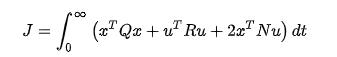
Here, Q is a matrix which tells us about the penalty that could be developed if x is not present as desired. We need to make the matrix Q quite big so that the pendulum is easily stabilised. The R vector tells us the penalty for the energy used. The R vector has to be small so that we can actuate it aggressively. When we have Q and R then we will have the K matrix (u=-Kx). This is the best control protocol that minimises the cost function and this is known as the Linear Quadratic Regulator control.
Simulation of pendulum system using LQR: Initial point: -pi/2 Stable at: pi lqr_pendulum
Simulation of spring-mass system using LQR: Initial point: (1,0) Stable at: (0,0) lqr_spring
Problems we faced during the simulations
As we are new to the MATLAB software, we weren’t well versed with the different functions and syntax that are used in it. To overcome this, we used the documentations provided by the users in the software itself for reference. This has helped us quite a lot. Along with this, we had quite a few errors while running our codes for which our mentors have been really helpful. Owing to these, we have been able to understand the working of this software in a better way and we hope to simulate other systems as well.
Future Tasks:
Our next task is to simulate a complex pulley ( also known as an atwood machine). For that, again we shall derive the Lagrangian equation and then move on with the animation and simulation part. Following which, we will stabilise an inverted pendulum using this software.